
Testing the tune package from tidymodels - analysing the relationship between the upsampling ratio and model performance
Have you ever also found yourself in a situation in which you were dealing with an imbalanced classification problem, but you weren’t really quite sure how much upsampling to apply? Or what’s exactly the impact of correcting the imbalance on model performance? In this post I will explore the relationship between the upsampling ratio and model performance, while using the brand new tidymodels tune package.
Introduction
Before doing any coding let’s start with a short introduction into the topic. Why should we account for class imbalance in the first place? The main reason for this is that otherwise it would be very difficult for any model to learn usefull patterns of the minority class from a dataset in which its exposure has a much lower frequency.
There’s also a number of techniques that could be used in order to combat class imbalance, but in this post I will not focus on covering all of them. Of course, the selection of the most appropriate method depends on a specific modelling task, so I would strongly suggest you get familiar with them. I am listing a couple good references below.
Coming back to the main question: what is the best value of the ratio to balance both target classes? Intuitively, it would be one that makes both classes equally frequent, but on the other hand, have you ever checked the impact of using different ratios on your model performance/ form? Wouldn’t it be great if we could easily simulate that and get all the results at hand? Thankfully we can easily do that with the use of the latest addition to the tidymodels stack called tune.
A bit of theory
I’ve wanted to write this post already a long time ago, because I’ve never found a direct and comprehensive answer to this question before. I hope I will be able to cover it well in this blogpost! Some of the more interesting resources that I came across online are listed below:
R Studio Community forum discussion - that was my first post on the topic, which eventually inspired me to write this blog, where I was discussing it with Max Kuhn. I will be addressing all those points below.
svds - very nice and comprehensive article that discusses ways of dealing with class imbalance. It’s a good place to get you started on the topic as it contains many references as well.
xgboost docs - xgboost creators argue that when the dataset it rebalanced in any way, we cannot further trust the estimated probabilities directly. That is very much in line with my experience so far, and I will present one method to alleviate that.
scikit-learn - discusses another solution to combat class imbalance that uses
case_weights, but I really liked the way they presented the impact of using such a technique on where the hyperplane is derived. This is exactly what I meant when I wrote about a model having a ‘better form’. Even though upsampling is a separate technique it will have a comparable impact on your model’s ability to appropriately capture minority patterns.google-developers - Google gives some guidance on class imbalance severity classification and presents a very interesting framework combining: first downsampling, followed by using case weights, so that the model is calibrated and produces true probabilities. That could be a very useful approach when dealing with really big data - then you can ‘afford’ to get rid of some majority class examples, while still keeping the model calibrated without doing any additional work.
Once equiped with some preliminary theory let’s dive into our simulation and see the effects ourselves!
Initial setup
Please note that most of tidymodels packages are still unstable and subject to change. It’s likely that in a couple weeks/ months parts of this blog could be outdated and would not execute. I will try to keep it up to date, but nevertheless, the outcomes of the simulation will still hold true.
First let’s install all required packages. I had to install development versions of dials, parsnip and tune from Github in order to get it to work.
### Install the development versions of these packages
# devtools::install_github("tidymodels/dials")
# devtools::install_github("tidymodels/parsnip")
# devtools::install_github("tidymodels/tune")
set.seed(42)
options(max.print = 150)

library(doFuture)
library(magrittr)
library(tidymodels)
library(parsnip)
library(dials)
library(tune)
One of the vignettes of tune suggests to parallelize computations while searching for optimal hyperparameter values. We can achieve that by using the doFuture package below.
all_cores <- parallel::detectCores(logical = FALSE)

registerDoFuture()
cl <- makeCluster(all_cores)
plan(cluster, workers = cl)
In the simulation I decided to use the credit_data dataset available in the recipes package, which depicts a well-known classification problem of defaulted vs. non-defaulted loans.
data("credit_data")

credit_data %<>%
  set_names(., tolower(names(.)))

glimpse(credit_data)
## Observations: 4,454
## Variables: 14
## $ status    <fct> good, good, bad, good, good, good, good, good, good, b…
## $ seniority <int> 9, 17, 10, 0, 0, 1, 29, 9, 0, 0, 6, 7, 8, 19, 0, 0, 15…
## $ home      <fct> rent, rent, owner, rent, rent, owner, owner, parents, …
## $ time      <int> 60, 60, 36, 60, 36, 60, 60, 12, 60, 48, 48, 36, 60, 36…
## $ age       <int> 30, 58, 46, 24, 26, 36, 44, 27, 32, 41, 34, 29, 30, 37…
## $ marital   <fct> married, widow, married, single, single, married, marr…
## $ records   <fct> no, no, yes, no, no, no, no, no, no, no, no, no, no, n…
## $ job       <fct> freelance, fixed, freelance, fixed, fixed, fixed, fixe…
## $ expenses  <int> 73, 48, 90, 63, 46, 75, 75, 35, 90, 90, 60, 60, 75, 75…
## $ income    <int> 129, 131, 200, 182, 107, 214, 125, 80, 107, 80, 125, 1…
## $ assets    <int> 0, 0, 3000, 2500, 0, 3500, 10000, 0, 15000, 0, 4000, 3…
## $ debt      <int> 0, 0, 0, 0, 0, 0, 0, 0, 0, 0, 0, 0, 2500, 260, 0, 0, 0…
## $ amount    <int> 800, 1000, 2000, 900, 310, 650, 1600, 200, 1200, 1200,…
## $ price     <int> 846, 1658, 2985, 1325, 910, 1645, 1800, 1093, 1957, 14…
In this specific example the severerity of class imbalance is actually pretty low (28% minority class frequency), and it probably would be also acceptable if it almost was disregarded, however, applying upsampling will surely improve the model form. Let’s find out!
round(prop.table(table(credit_data$status)), 2)
##
##  bad good
## 0.28 0.72
Note that apart from regular train/ test splits I also decided to repeat the CV process three times. The dataset isn’t particularly big so we can get more stable and reliable results by performing the CV process more than once.
split <- initial_split(credit_data, prop = 0.80, strata = "status")

df_train <- training(split)
df_test  <- testing(split)

(train_cv <- vfold_cv(df_train, v = 5, repeats = 3, strata = "status"))
## #  5-fold cross-validation repeated 3 times using stratification
## # A tibble: 15 x 3
##    splits             id      id2
##    <named list>       <chr>   <chr>
##  1 <split [2.9K/714]> Repeat1 Fold1
##  2 <split [2.9K/713]> Repeat1 Fold2
##  3 <split [2.9K/713]> Repeat1 Fold3
##  4 <split [2.9K/713]> Repeat1 Fold4
##  5 <split [2.9K/712]> Repeat1 Fold5
##  6 <split [2.9K/714]> Repeat2 Fold1
##  7 <split [2.9K/713]> Repeat2 Fold2
##  8 <split [2.9K/713]> Repeat2 Fold3
##  9 <split [2.9K/713]> Repeat2 Fold4
## 10 <split [2.9K/712]> Repeat2 Fold5
## 11 <split [2.9K/714]> Repeat3 Fold1
## 12 <split [2.9K/713]> Repeat3 Fold2
## 13 <split [2.9K/713]> Repeat3 Fold3
## 14 <split [2.9K/713]> Repeat3 Fold4
## 15 <split [2.9K/712]> Repeat3 Fold5
Model specification
I will use parsnip as the main modelling engine and decided to train a regular Random Forest model. I wanted to select a model that has already embedded regularization, but doesn’t require a lot hyperparameter tuning to provide a good solution. The reason for that is we need to keep our model parameters constant and tune the value of oversampling - otherwise our results would not be comparable.
(engine <- rand_forest(
  mtry = 2,
  trees = 500,
  min_n = 10
  ) %>%
  set_mode("classification") %>%
  set_engine("ranger"))
## Random Forest Model Specification (classification)
##
## Main Arguments:
##   mtry = 2
##   trees = 500
##   min_n = 10
##
## Computational engine: ranger
The next step is to specify our modelling recipe. It’s a pretty standard one that definitely
could be further modified to improve model performance, but one thing is definitely worth
pointing out - the usage of tune() in the last line. It’s used as a placeholder for a set of candidate values that will be evaluated. That’s how we can add information
to our recipe/ model tuning process about a parameter that will need to be optimized during fitting.
recipe <- df_train %>%
  recipe(status ~ .) %>%

  # Imputation: assigning NAs to a new level for categorical
  # (that's good practice, but not needed here) and median imputation for numeric
  step_unknown(all_nominal(), -status) %>%
  step_medianimpute(all_numeric()) %>%

  # Combining infrequent categorical levels and introducing a new level
  # for prediction time (that's good practice, but not needed here)
  step_other(all_nominal(), -status, other = "infrequent_combined") %>%
  step_novel(all_nominal(), -status, new_level = "unrecorded_observation") %>%

  # Hot-encoding categorical variables
  step_dummy(all_nominal(), -status, one_hot = TRUE) %>%

  # Creating additional ratio variables - they typically make sense
  # in credit scoring problems
  step_mutate(
    ratio_expenses_income = expenses / (income + 0.001),
    ratio_assets_income = assets / (income + 0.001),
    ratio_debt_income = debt / (income + 0.001),
    ratio_debt_assets = debt / (assets + 0.001),
    ratio_amout_price = amount / (price + 0.001)
  ) %>%

  # Adding upsampling
  step_upsample(status, over_ratio = tune())
Now I’m using the dials package to create a grid of candidate values for the upsampling ratio, which will be evaluated during model fitting. Based on recipes::step_upsample() documentation we can see that an upsampling ratio value equal to 1 means, that all target levels are sampled to have the same frequency. A value of 0.5 would mean that the minority class will be half as frequent as the majority class (approximately).
(grid <- grid_regular(
  over_ratio() %>% range_set(c(0.5, 1.5)),
  levels = 11
  ))
## # A tibble: 11 x 1
##    over_ratio
##         <dbl>
##  1        0.5
##  2        0.6
##  3        0.7
##  4        0.8
##  5        0.9
##  6        1
##  7        1.1
##  8        1.2
##  9        1.3
## 10        1.4
## 11        1.5
Let’s move to the final step of connecting all previously specified inputs: our recipe, model engine, resampled train/ test sets and grid of candidate values to evaluate. On top of that we pass which metrics we would like to track for each iteration using the yardstick package, as well as disable verbosity of the procedure. Note that in the grid_control function call parallel processing is enabled by default if a parallel backend is registered.
Please keep in mind that even though we’re running this in parallel, this code chunk will most probably execute for a couple of minutes before all models will be fitted. The outcome of the tune_grid function is a tidy, nested tibble object separated by CV repetition and each hold-out fold performance metrics requested in the call.
(fits <- tune_grid(
  recipe,
  model = engine,
  rs = train_cv,
  grid = grid,
  perf = metric_set(roc_auc, j_index, sens, spec),
  control = grid_control(verbose = FALSE)
  ))
## #  5-fold cross-validation repeated 3 times using stratification
## # A tibble: 15 x 5
##    splits             id      id2   .metrics          .notes
##  * <list>             <chr>   <chr> <list>            <list>
##  1 <split [2.9K/714]> Repeat1 Fold1 <tibble [44 × 4]> <tibble [0 × 1]>
##  2 <split [2.9K/713]> Repeat1 Fold2 <tibble [44 × 4]> <tibble [0 × 1]>
##  3 <split [2.9K/713]> Repeat1 Fold3 <tibble [44 × 4]> <tibble [0 × 1]>
##  4 <split [2.9K/713]> Repeat1 Fold4 <tibble [44 × 4]> <tibble [0 × 1]>
##  5 <split [2.9K/712]> Repeat1 Fold5 <tibble [44 × 4]> <tibble [0 × 1]>
##  6 <split [2.9K/714]> Repeat2 Fold1 <tibble [44 × 4]> <tibble [0 × 1]>
##  7 <split [2.9K/713]> Repeat2 Fold2 <tibble [44 × 4]> <tibble [0 × 1]>
##  8 <split [2.9K/713]> Repeat2 Fold3 <tibble [44 × 4]> <tibble [0 × 1]>
##  9 <split [2.9K/713]> Repeat2 Fold4 <tibble [44 × 4]> <tibble [0 × 1]>
## 10 <split [2.9K/712]> Repeat2 Fold5 <tibble [44 × 4]> <tibble [0 × 1]>
## 11 <split [2.9K/714]> Repeat3 Fold1 <tibble [44 × 4]> <tibble [0 × 1]>
## 12 <split [2.9K/713]> Repeat3 Fold2 <tibble [44 × 4]> <tibble [0 × 1]>
## 13 <split [2.9K/713]> Repeat3 Fold3 <tibble [44 × 4]> <tibble [0 × 1]>
## 14 <split [2.9K/713]> Repeat3 Fold4 <tibble [44 × 4]> <tibble [0 × 1]>
## 15 <split [2.9K/712]> Repeat3 Fold5 <tibble [44 × 4]> <tibble [0 × 1]>
The outcome can be further easily summarized with the estimate function, which will extract and flatten the .metrics column. That makes it very convenient to visualize the performance profile of the model.
estimate(fits) %>%
  arrange(desc(over_ratio))
## # A tibble: 44 x 6
##    over_ratio .metric .estimator  mean     n std_err
##         <dbl> <chr>   <chr>      <dbl> <int>   <dbl>
##  1        1.5 j_index binary     0.510    15 0.0103
##  2        1.5 roc_auc binary     0.837    15 0.00421
##  3        1.5 sens    binary     0.699    15 0.00919
##  4        1.5 spec    binary     0.812    15 0.00471
##  5        1.4 j_index binary     0.512    15 0.0104
##  6        1.4 roc_auc binary     0.837    15 0.00437
##  7        1.4 sens    binary     0.701    15 0.00881
##  8        1.4 spec    binary     0.811    15 0.00479
##  9        1.3 j_index binary     0.514    15 0.0107
## 10        1.3 roc_auc binary     0.838    15 0.00410
## # … with 34 more rows
Analyzing performance profile
For visualization of the results I will use my own ggrapid package that you can install from Github. After having a quick look at the plot we can arrive at the following conclusions:
library(ggrapid)

estimate(fits) %>%
  mutate(
    over_ratio = as.character(over_ratio)
    ) %>%
  rename(
    Metric = .metric
  ) %>%
  plot_line(
    over_ratio,
    mean,
    fill = Metric,
    title = "Performance metrics across different upsampling ratio values",
    caption = "Upsampling ratio = 1 - equal classes frequency",
    lab_x = "Upsampling ratio between both classes",
    lab_y = "Performance metric value",
    angle = 0,
    limit_max = 1
    )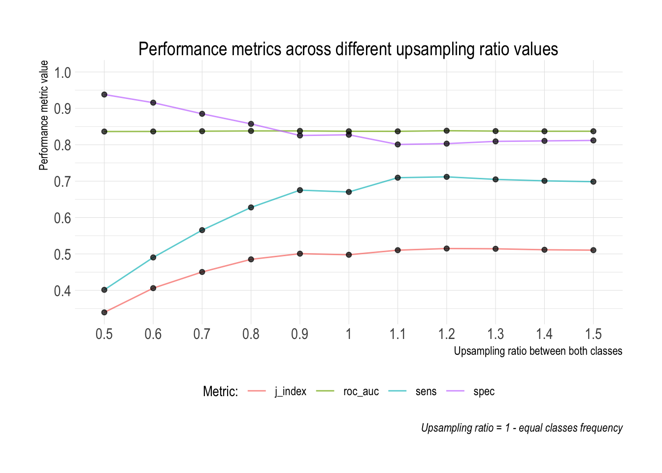
ROC AUC - regardless of the value of the upsampling ratio the overall rank ordering ability of the model remains constant. It makes sense as the ROC AUC is calculated across the entire space of probability cut-offs.
Sensitivity / specificity - with a higher value of the upsampling ratio sensitivity increases, while specificity decreases. This shows that even though the overall ability of the model remains constant (point above), itss inner workings and ability to better capture the patterns of the minority class significantly improve. This is precisely what we want to achieve in problems such as credit scoring. The main reason for this is that both types of errors have vastly different associated costs.
J-index - confirms the previous point as it’s calculated as: sensitivity + specificity - 1. The J-index suggests that the best trade-off between sensitivity and specificity is achieved when the upsampling ratio is equal to 1.1. In practice it means that the frequency of the minority class is by 10% higher than the majority class.
The above analysis proves that even though there is no impact of upsampling on the ROC AUC, combatting class imbalance has an enourmous impact on how the minority patterns are exposed and eventually learnt by the algorithm.
Most software packages and tools by default suggest an upsampling ratio that makes both frequencies equal - it makes a lot of sense and is a reasonable default. What’s surprising though is that (at least for this example) we can see that the best model form is obtained with an upsampling ratio equal to 1.1.
Can we trust upsampled probabilities?
If you thought that’s the end if this post you were wrong. The reason for this is that estimated probabilities from upsampled models can’t be trusted and used directly by decision makers (as also pointed in XgBoost documentation). Check out the next chunks to find out why!
First of all, let’s extract the value of the upsampling ratio that resulted in the best model form. Our goal now is to fit the model to the entire training set using that best parameter value.
(over_ratio_best <- estimate(fits) %>%
  filter(.metric == "j_index") %>%
  arrange(desc(mean)) %>%
  slice(1) %>%
  pull(over_ratio))
## [1] 1.2
Now we need to update our originally specified recipe using the update function. Perhaps there will be a better way of doing that in the upcoming tidymodels stack, but that was the best method I was able to find at the moment of writing this post.
recipe_best <- recipe
recipe_best$steps[[7]] <- update(recipe$steps[[7]], over_ratio = over_ratio_best)
Once we have the recipe updated, we prep it and use fit on our previously specified Random Forest engine.
recipe_best_prep <- prep(recipe_best, retain = TRUE)

(fit_best <- engine %>%
  fit(status ~ ., juice(recipe_best_prep)))
## parsnip model object
##
## Ranger result
##
## Call:
##  ranger::ranger(formula = formula, data = data, mtry = ~2, num.trees = ~500,      min.node.size = ~10, num.threads = 1, verbose = FALSE, seed = sample.int(10^5,          1), probability = TRUE)
##
## Type:                             Probability estimation
## Number of trees:                  500
## Sample size:                      6146
## Number of independent variables:  34
## Mtry:                             2
## Target node size:                 10
## Variable importance mode:         none
## Splitrule:                        gini
## OOB prediction error (Brier s.):  0.1298593
And now’s the main point - if no upsampling was performed, we could use that model as is and obtain reliable predictions. But having used a rebalancing technique, the estimated model probabilities follow now a different distribution.
If you recall, the frequency of the minority class was roughly 28%, therefore the average estimated probability of the model should be almost identical. However, the average estimated probability of our model is now 0.4279812!
It means that these probabilities can’t be used by any decision makers directly, because they have a completely different distribution than our original training data. Can we do anything about that?
df_train_pred <-
  df_train %>%
  select(status) %>%
  mutate(
    prob = predict(fit_best, bake(recipe_best_prep, df_train), "prob") %>%
      pull(.pred_bad)
  )

mean(df_train_pred$prob)
## [1] 0.4279812
Probabilities calibration
A very usefull technique that can help us in this situation is called Platt’s scaling. I do not want to get too deep into explaining probabilities calibration in this post, but go ahead and check out that link to get to know more.
However, just to give a high level overview: the point of probabilities calibration is to scale estimated model probabilities back to their original distribution (with same or different mean). You can perform probabilities scaling with Platts using the function below that I once implemented in one of my packages.
calibrate_probabilities <- function(df_pred,
                                    target,
                                    prediction,
                                    top_level = "1",
                                    target_prob = 0.0
                                    ) {

  var_target <- rlang::enquo(target)
  var_prediction <- rlang::enquo(prediction)

  df_pred <- df_pred %>%
    mutate(
      target = case_when(
        !!var_target == top_level ~ 1,
        TRUE ~ 0),
      score = round(100 * log((1 - !!var_prediction) / !!var_prediction), 0)
      )

  glm <- stats::glm(target ~ score, data = df_pred, family = "binomial")
  glm_coef <- glm$coef

  dr <- nrow(filter(df_pred, !!var_target == top_level)) / nrow(df_pred)
  target_prob <- ifelse(target_prob == 0, dr, target_prob)
  k <- (dr / (1 - dr)) / (target_prob / (1 - target_prob)) # final scaling factor

  df_pred %<>%
    mutate(
      prediction_scaled = 1 / (1 + k * exp(-(glm_coef[[1]] + glm_coef[[2]] * score)))
    )

  list(
    glm_fit = glm,
    glm_coef = glm_coef,
    parameters = list(
      dr = dr,
      target_prob = target_prob,
      k = k
    ),
    df_calibrated = df_pred
    )

}
Let’s put the function into practice and check the results:
calibration <- calibrate_probabilities(
df_train_pred,
status,
prob,
"bad"
)
mean(calibration$df_calibrated$prediction_scaled)
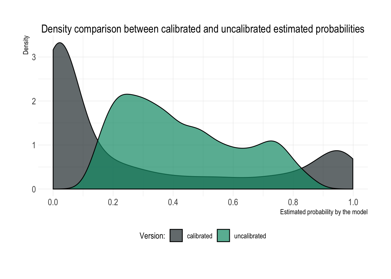
## [1] 0.2816269Great! We scaled our estimated probabilities back to the original distribution and we’re getting back the original minority class frequency as the average estimated probability value. In case you’re still not convinced, take a look at the comparison of distributions between both estimated probabilities presented below.
The upsampled distribution of probabilities is definitely less pathological and normal-looking than the original one, but unfortunately it no longer represents business reality. Therefore, if you are planning to expose raw probabilities directly in any of your applications to people that are supposed to make decisions based on them, you need to calibrate them back to their original distribution (grey colour).
df_train_pred %>%
  mutate(version = "uncalibrated") %>%
  bind_rows(
    calibration$df_calibrated %>%
      select(
        status,
        prediction_scaled
      ) %>%
      rename(prob = prediction_scaled) %>%
      mutate(version = "calibrated")
  ) %>%
  plot_density(
    prob,
    fill = version,
    title = "Density comparison between calibrated and uncalibrated estimated probabilities",
    lab_x = "Estimated probability by the model",
    quantile_low = 0,
    quantile_high = 1
    )
Wrapping up
Ok, that was a pretty long post but I hope that some of you will find it useful, and that perhaps it will save some of you the time of searching through the internet for answers that I was once looking for! As the main takeaway - remember that pretty much after any rebalancing you need to calibrate your probabilities back to their original distribution, if they are intended to be interpreted directly by any decision makers.
Also I need to admit that I’m really very impressed with the progress the R Studio Team is making on the tidymodels stack. I’m pretty sure that eventually the R community will finally have a very comprehensive, complete and consistent stack of tools to build and validate all sorts of Data Science & Machine Learning solutions. Thank you!